Trophic Functions in Predator–Prey Models

20 min., 1/3

Mathematical models play an invaluable role in studying nature. These models not only allow us to predict future developments, but they also serve several other important purposes.

The use of ecological models is sometimes referred to as applying physical methods in ecology, since ecosystems are studied in terms of population dynamics using mathematical techniques originally developed for solving problems in physics. The outputs of such models can provide insights such as the following:

• Prediction. The ability to work with mathematical models of ecosystems makes it possible to forecast future developments. These may concern a stable environment or one in which certain parameters are changing. Understanding the model then allows us to assess how such changes will affect the ecosystem.
• Understanding Principles. Mathematical models help ecologists and scientists examine the interactions between various components of ecosystems and gain insight into their dynamics. This in turn helps identify the factors that shape the structure and function of these ecosystems.
• Decision-making Optimization. Mathematical modelling can also be used to improve decision-making in areas such as biodiversity conservation or the management of forests and fisheries. It helps identify the most effective strategies to achieve specific goals.

One of the fundamental ecological relationships is the predator–prey interaction. This relationship may be the only interaction in a given ecosystem, or it may be accompanied by others. The importance of modelling predator–prey coexistence will be illustrated using several historically significant models.

The Lotka-Volterra Model

In 1926, Italian mathematician Vito Volterra published one of the first mathematical models of predator–prey interactions. He was motivated by an observation made during World War I, when fishing restrictions led to an increased percentage of predatory fish in the catch. This surprising trend was pointed out to Volterra by his son-in-law, marine biologist Umberto D’Ancona, who had expected the opposite: he assumed that reduced fishing pressure would increase the proportion of smaller fish species, which serve as prey for predators. Volterra’s model explained this phenomenon as a result of simple interactions between predatory fish and their prey.

The model consists of two equations. The first describes the prey population, assuming that it grows naturally, but this growth is limited by the presence of predators. A higher number of predators slows the prey population’s growth more significantly. If there are too many predators, the prey population may even begin to decline and eventually go extinct. The second equation describes the predator population. It assumes that without prey, the predators die out. However, the more prey is available, the more this trend reverses, allowing the predator population to grow.

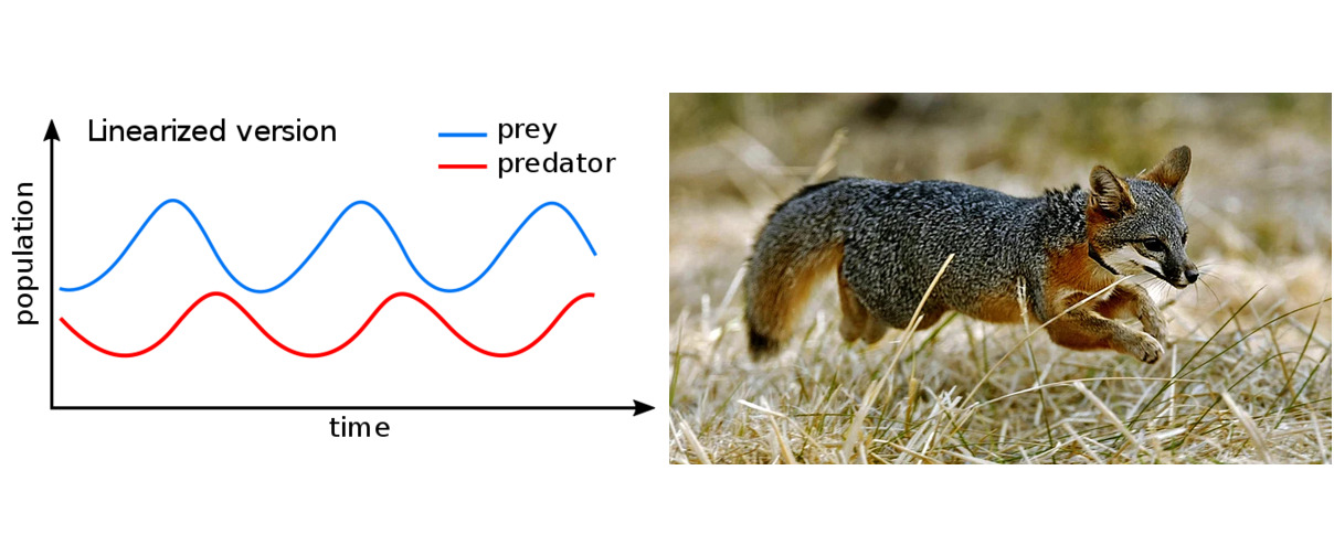
This system naturally produces cycles. An abundance of prey allows the predator population to increase. As predator numbers grow, they put increasing pressure on the prey population, eventually driving it to decline. This leads to a food shortage for predators, which in turn causes a decline in their own numbers. Eventually, the predator population becomes so small that the prey population experiences less pressure and can grow again, eventually reaching its original level. This, in turn, allows the predator population to recover, and the cycle repeats. These periodic fluctuations in population sizes can be clearly observed in historical fur-trade records of snowshoe hares and lynxes in the Hudson Bay area.

Volterra’s model explained not only the emergence of such cycles, but also why restricting hunting or fishing can shift the equilibrium point—around which both populations oscillate—in favor of the predator rather than the prey. This phenomenon, observed by D’Ancona, is known as the Volterra effect.

The same model had actually been proposed earlier, in 1910, by American mathematician Alfred J. Lotka. For this reason, it is now known as the Lotka–Volterra model.

The Spruce Budworm Model

Similar periodic fluctuations as those described by the Lotka–Volterra model can also be observed in Canadian forests. Approximately every 30 to 40 years, there has been a massive outbreak of the spruce budworm (Choristoneura fumiferana). This moth species typically exists in relatively low numbers, but in certain years, its population increases by a factor of a thousand. During such outbreaks, the larvae can destroy up to 80% of the trees in a forest, effectively devastating the entire area. One of the most recent large-scale infestations began in 2006 in Quebec. By 2019, around 9.6 million hectares of forest ¹ had been affected—an area larger than the size of Hungary.

In 1978, scientists D. Ludwig, D. D. Jones, and C. S. Holling proposed a model that not only described the population dynamics of the spruce budworm but also helped explain the mechanisms behind these outbreaks. The key factor was predation—specifically, birds feeding on the budworm larvae. In the natural ecosystem, birds helped keep the budworm population in check, but only up to a certain point. Once the forest had grown large enough, it provided ample food for the budworms as well. Their population then increased so much that the birds became saturated and could no longer consume larvae at a rate sufficient to limit their numbers. As a result, the birds’ role as predators diminished, and the budworm population exploded, ultimately causing extensive forest damage.

In this case, predation plays a crucial role in limiting the budworm population. However, because birds reproduce much more slowly than budworms, their population can be considered constant for modelling purposes. Once birds reach their saturation point, they can only reduce the budworm population growth to a limited extent. Beyond a certain threshold, this control becomes ineffective, leading to uncontrolled population growth and a full outbreak.

The Island Fox Model

The island fox (Urocyon littoralis) is a unique species, an endemic mammal that lives only on a few small islands off the coast of California. Roughly the size of a domestic cat, the island fox is unusually trusting due to the absence of natural predators in its habitat. As a species, it is highly sensitive and vulnerable, with low genetic variability and limited resistance to diseases introduced from the mainland. It is one of the smallest canids in the world, and unlike most other members of the dog family, it can climb trees.

Due to human activity, the island fox population declined dramatically around the turn of the millennium. On San Miguel Island, the number of adult individuals dropped from 450 in 1994 to just 15 in 1999². A similar situation occurred on the surrounding islands, each of which is home to its own subspecies of island fox. The decline was caused by a chain of events: the production of the insecticide DDT in the 1940s led to the extinction of bald eagles (Haliaeetus leucocephalus) in the area. In their absence, golden eagles (Aquila chrysaetos) moved in. Unlike the fish-eating bald eagle, the golden eagle prefers mammals, which proved catastrophic for the island fox. Once the top predator on the islands, the fox suddenly became prey—and by the early 2000s, the species was on the brink of extinction. Unlike in the Lotka–Volterra model, there was no hope that the fox population would naturally rebound due to predator–prey oscillations, because the eagles had alternative food sources such as wild pigs and skunks.

Fortunately, the island fox was saved through an extraordinary conservation effort. Once the causes of the decline were correctly identified, the recovery could begin. Conservationists focused on increasing the fox population and stabilizing its environment. This involved eradicating wild pigs, relocating golden eagles, reintroducing bald eagles, breeding foxes in captivity, releasing them into the wild, and vaccinating them against introduced diseases. All of this was achieved in record time—within a single decade. It became one of the most successful mammal recovery programs in history.

Trophic Functions

An essential component of predator–prey models—regardless of which of the above examples we consider—is the trophic function. This function describes the effect of a single predator on a prey population. It expresses the rate at which one predator slows the growth of the prey population. If we let \(x\) be the size of the prey population and \(y\) the rate at which one predator slows the prey’s growth (i.e., the amount of prey caught by one predator per unit of time), then this relationship can be written mathematically as: \[y=f(x).\] We will try to identify some natural assumptions that any trophic function should meet. Then we will attempt to find a suitable general form of such a function.

Solution.

1. The function \(y=f(x)\) is increasing.

2. The function \(y=f(x)\) goes through the origin, i.e., \(f(0)=0\).

3. The function \(y=f(x)\) is bounded above. Since the function is increasing and is bounded above, its graph has a horizontal asymptote as \(x\) approaches infinity.

Holling Type II Trophic Function

The trophic function expresses how much prey a single predator consumes per unit time, given the size of the prey population. Therefore, the function must be defined for non-negative values only, and its outputs must also be non-negative (this follows from points 1 and 2 in the previous exercise). In the previous section, we established that the trophic function should pass through the origin and grow toward a horizontal asymptote—that is, the function should increase but be bounded above. These properties cannot be met by a linear function, so we turn to the simplest nonlinear case: an inverse proportionality.

Solution.

1. The function obtained by vertically scaling \(y=\frac{1}{x}\) by a factor of \(k\) is: \[y=\frac{k}{x}.\]

2. The inversion is achieved by multiplying the function by a factor of \(-1\) and the shift is achieved by by adding the value of \(S\). These adjustments give the function \[y=S-\frac{k}{x}.\]

3. The shift to the left by \(b\) is achieved by substituting the expression \(x+b\) for \(x\). This gives us the function \[y=S-\frac{k}{x+b}.\] When converted to the common denominator the function takes the form \[y=\frac{Sx+Sb}{x+b}-\frac{k}{x+b}=\frac{Sx + (Sb-k)}{x+b}.\] To ensure \(f(0)=0\), we must have: \[Sb-k=0\]. This condition shows that the three constants are not independent, but there is a relationship between them.

Note. In the previous exercise, we derived the general form of one of the basic trophic functions. It is an increasing function that starts at the origin and gradually grows toward a horizontal asymptote. The growth rate slows down over time. Such a function is called the _Holling Type II function. It is commonly written in the form: \[f(x)=\frac {Sx}{x+b} (1),\tag{1}\] where \(S\) is the saturation level and \(b\) is a constant whose meaning will be explained in the next exercise.

Solution. By directly substituting \(x=b\) into (1), we get \[ f(b)=\frac{Sb}{b+b}=\frac {Sb}{2b}=\frac S2. \] This proves the statement.

The following exercise illustrates the reverse process, where from a trophic function in form (1) we will derive a form that reveals how it can be obtained through successive transformations of the function \(y=\frac {1}{x}\).

Solution. To solve this, we cleverly rewrite the fraction. In the numerator, we create a multiple of the denominator, split the expression into two fractions, and simplify:

\[\frac {6x}{x+2} = \frac {6(x+2)-12}{x+2}=\frac {6(x+2)}{x+2}-\frac {12}{x+2}=6-12\frac 1{x+2}\]

This calculation shows that the graph of the given function is obtained by scaling the graph of the function \(y=\frac{1}{x}\) vertically by a factor of 12, by inverting it around the horizontal axis, shifting it 6 units upward and 2 units to the left.

The same result could also be obtained by performing polynomial division of the numerator by the denominator.

Solution. From the note before Exercise 3, we know the general form of the trophic function is: \[ y=\frac{Sx}{x+b}, \] where \(S\) is the saturation value of the predator, so we substitute \(S=6\): \[ y=\frac{6x}{x+b}\,. \] We can tell the value of the parameter \(b\) straight away based on the result of Exercise 3, but we can also quickly compute it from the second condition in the problem statement. We know that \[ 3=\frac{6\cdot 210}{210+b} \] and from there we get \(b=210\). So the final form of the function is \[ y=\frac{6x}{x+210}\,. \]

References

Literature

• Wikipedia, https://en.wikipedia.org/wiki/Lotka%E2%80%93Volterra_equations March 3, 2024
• R Mařík, Dynamické modely populací (in Czech), https://robert-marik.github.io/dmp/uvod.html, March 3, 2024
• D. Ludwig, D.D. Jones, C.S. Holling: Qualitative analysis of insect outbreak systems: the spruce budworm and forest, Journal of Animal Ecology 47(1): 315–332, February 1978.

Image Sources

• https://en.wikipedia.org/wiki/Lotka%E2%80%93Volterra_equations#/media/File:Lotka_Volterra_dynamics.svg
• https://www.npr.org/sections/thetwo-way/2016/08/11/489695842/once-nearly-extinct-california-island-foxes-no-longer-endangered Kevork Djansezian/AP