
Linear Regression
 30 min.,
  2/3
2/3 In practice, we often encounter situations where the values of one variable determine the values of another. Based on a set of measured or statistically obtained data, we then try to find a mathematical model that describes the functional relationship between the two variables. For example, consider data indicating the height and weight of American women aged between 30 and 39 (source: https://en.wikipedia.org/wiki/Simple_linear_regression, accessed April 12, 2024; for brevity, only half of the data is used).
| height/m | \(1{.}47\) | \(1{.}52\) | \(1{.}57\) | \(1{.}63\) | \(1{.}68\) | \(1{.}73\) | \(1{.}78\) | \(1{.}83\) |
|---|---|---|---|---|---|---|---|---|
| weight/kg | \(52{.}21\) | \(54{.}48\) | \(57{.}20\) | \(59{.}93\) | \(63{.}11\) | \(66{.}28\) | \(69{.}92\) | \(74{.}46\) |
The data is displayed in the figure on the left. It is evident from the figure that as height increases, weight also tends to increase. In such a case, it is possible to find a mathematical model that expresses weight as a function of height. Such a mathematical model is shown in color in the figure on the right. It allows us to predict a woman’s weight based on her height.

The type of problem described above is called linear regression.
Linear regression is one of the fundamental methods in machine learning. It involves identifying a functional relationship hidden within a set of data. Once we have this relationship, we can use it to predict function values for inputs that are not included in the original dataset.
In the following section, we will show how linear regression is related to linear combinations of vectors, and how the regression line can be found using vector operations. We will proceed step by step:
- First, we will review how to express a vector as a linear combination of given vectors.
- Then, we will see how this task can be simplified if one of the vectors is perpendicular to the others.
- Next, we will explore how to find an approximate solution when an exact one does not exist.
- Finally, we will use these ideas to solve the problem of linear regression — that is, we will construct a mathematical model based on the given data that reveals the underlying trend and allows us to make predictions for values not present in the dataset.
Linear Combination of Vectors
Exercise 1. Express the vector \(\vec c = \begin{pmatrix}1 \cr 2\end{pmatrix}\) as a linear combination of the vectors \(\vec a = \begin{pmatrix}2 \cr 2\end{pmatrix}\) and \(\vec b = \begin{pmatrix}3 \cr 1\end{pmatrix}\).
Solution. Expressing the vector \(\vec c\) as a combination of the vectors \(\vec a\) and \(\vec b\) means finding numbers \(t_1\) and \(t_2\) such that \[ t_1 \vec a + t_2 \vec b = \vec c. \] Writing this out in coordinates leads to the following system of equations: \[ \begin{aligned} 2t_1+3t_2 &= 1,\cr 2t_1+t_2 &=2. \end{aligned} \] This system has a unique solution: \(t_1=\frac 54\) and \(t_2=-\frac 12\).
Exercise 2. Express the vector \(\vec w=\begin{pmatrix}1\cr 2\cr 1\end{pmatrix}\) as a linear combination of the vectors \[ \vec u_1=\begin{pmatrix}2\cr 2\cr 1\end{pmatrix},\quad \vec u_2=\begin{pmatrix}3\cr 1\cr 2\end{pmatrix},\quad \vec u_3=\begin{pmatrix}3\cr -1\cr -4\end{pmatrix}. \]
Solution. As in the previous problem, we are looking for numbers \(t_1\), \(t_2\) and \(t_3\) such that \[ t_1 \vec u_1+t_2\vec u_2 + t_3 \vec u_3 = \vec w.\tag{1} \] Substituting the coordinates gives a system of three equations with three unknowns \[\tag{2} \begin{aligned} 2t_1 + 3t_2 + 3t_3 &= 1,\cr 2 t_1 + t_2 -t_3 &=2,\cr t_1+2t_2-4t_3&=1. \end{aligned} \] Solving such a system is already somewhat tedious, but using the method of substitution or elimination, we find: \[ t_1=\frac{14}{13},\quad t_2=-\frac{7}{26},\quad t_3=-\frac{3}{26}. \]
Linear Combination Using the Dot Product
If at least one of the given vectors is perpendicular to the remaining vectors, we can use a clever trick to obtain a simpler system of equations.
Let’s go back to the previous problem. We can observe that the vector \(\vec u_3\) is perpendicular to the vectors \(\vec u_1\) and \(\vec u_2\). This means it is also perpendicular to the plane defined by these two vectors. We can easily verify this by calculating the dot products: \[ \vec u_1\cdot \vec u_3 = 2\cdot 3 +2\cdot (-1)+1\cdot (-4) = 0 \] and \[ \vec u_2\cdot \vec u_3 = 3\cdot 3 +1\cdot (-1)+2\cdot (-4) = 0. \] Thanks to this property, it is worth multiplying equation (1) using dot product by the vectors \(\vec u_1\) to \(\vec u_3\). This gives us the following three equations. \[ \begin{aligned} t_1 (\vec u_1\cdot \vec u_1) + t_2 (\vec u_2\cdot \vec u_1) + t_3 (\vec u_3\cdot \vec u_1) &= \vec w\cdot \vec u_1\cr t_1 (\vec u_1\cdot \vec u_2) + t_2 (\vec u_2\cdot \vec u_2) + t_3 (\vec u_3\cdot \vec u_2) &= \vec w\cdot \vec u_2\cr t_1 (\vec u_1\cdot \vec u_3) + t_2 (\vec u_2\cdot \vec u_3) + t_3 (\vec u_3\cdot \vec u_3) &= \vec w\cdot \vec u_3 \end{aligned} \] By calculating the dot products, we obtain a system that is much simpler than system (2). \[ \begin{aligned} 9t_1+10t_2=7\cr 10t_1+14t_2=7\cr 26t_3=-3 \end{aligned} \] From the last equation, we can directly determine one of the unknowns, and the first two equations form a system of two equations with two unknowns, \(t_1\) and \(t_2\).
Linear Combinations and Inconsistent Systems of Equations
Let us recall that a system of linear equations is said to be inconsistent if it has no solution.
We will now modify our previous problem involving the expression of a vector as a linear combination of given vectors. This time, we will omit one of the vectors we previously used. As a result, the problem becomes unsolvable in the classical sense.
Exercise 3. Express the vector \(\vec w=\begin{pmatrix}1\cr 2\cr 1\end{pmatrix}\) as a linear combination of the vectors \[ \vec u_1=\begin{pmatrix}2\cr 2\cr 1\end{pmatrix},\quad \vec u_2=\begin{pmatrix}3\cr 1\cr 2\end{pmatrix}. \]
Solution. We need to find numbers \(t_1\), \(t_2\) such that \[t_1\vec u_1 + t_2\vec u_2 = \vec w.\] Writing this out in coordinates leads to the following system: \[ \begin{aligned} 2t_1 + 3t_2 &= 1,\cr 2 t_1 + t_2 &=2,\cr t_1+2t_2&=1. \end{aligned} \] It is easy to verify that this system is inconsistent and has no solution. Indeed, we already solved the system consisting of the first two equations earlier (\(t_1=\frac 54\) and \(t_2=-\frac 12\)), and the last equation conflicts with these values (\(\frac 54+2\cdot(-\frac 12)\neq 1\)).
Solving an Inconsistent System of Equations
Let us now introduce a reasonable generalization of what we consider a solution. Instead of searching for values of the unknowns that make the left- and right-hand sides exactly equal, we will look for values that make the two sides as close to each other as possible.
By the solution of an inconsistent system of equations we will mean a choice of the unknowns for which the length of the vector expressing the difference between the left- and right-hand sides of the system is minimal.
The accompanying figure helps us understand what this system represents and how to visualize its solution in the weakened sense described above.

This combination is given by the vector \(\vec w_0\), and the difference between \(\vec w\) and \(\vec w_0\) is represented by the vector \(\vec \varepsilon\). Our goal is to make the length of the vector \(\vec \varepsilon\) as small as possible.
From a visual point of view and geometric properties, it is easy to see that this occurs when the vector \(\vec \varepsilon\) is perpendicular to the plane defined by the vectors \(\vec u_1\) and \(\vec u_2\). This brings us to the same situation we encountered in the alternative solution to Exercise 3. There, we also used a trick to find the coefficients of \(\vec u_1\) and \(\vec u_2\) without solving the full system of equations—we took the dot product of the system with the vectors \(\vec u_1\) and \(\vec u_2\). In fact, we didn’t even need to know the vector \(\vec \varepsilon\) for this calculation.
Since the length of the vector \(\vec \varepsilon\) is expressed in terms of the squares of its components, this method is called the least squares method.
We will demonstrate the entire procedure using the following example.
Linear Regression
Let us consider the data in the following table:
| \(x\) | \(2\) | \(3\) | \(4\) |
|---|---|---|---|
| \(y\) | \(1\) | \(5\) | \(7\) |
We are looking for a line \(y=ax+b\) that best captures the trend in this dataset and serves as a suitable mathematical model for the data. By substituting each of the three points into the equation of the line, we obtain a system of three equations in two unknowns. \[ \begin{aligned} 2a+b=1\cr 3a+b=5\cr 4a+b=7 \end{aligned} \] This is a system of equations that is inconsistent — also known as an overdetermined system — and it has no solution in the classical sense. The vector form of the system is: \[ a \begin{pmatrix}2\\3\\4\end{pmatrix} + b \begin{pmatrix}1\\1\\1\end{pmatrix} = \begin{pmatrix}1\\5\\7\end{pmatrix} \] Taking the dot product of both sides with the vectors \(\begin{pmatrix}2\\3\\4\end{pmatrix}\) and \(\begin{pmatrix}1\\1\\1\end{pmatrix}\) gives the following system of two equations: \[ \begin{aligned} 29a+9b&=45\\ 9a+3b&=13 \end{aligned} \] The solution to this system is \(a=3\) and \(b=-\frac {14}3\). The regression model for the given data is therefore the line \[y=3x-\frac {14}3.\] A graph containing the given data and the regression line is shown in the figure.

Regression for Larger Data Sets
The procedure described in the previous section for three points can be generalized to any number of points. It is not uncommon to work with data sets containing hundreds of points.
If the vector \(\vec X\) contains the values of the independent variable1 and the vector \(\vec Y\) contains the values of the dependent variable, we consider the model2 \[ \vec Y = a\vec X+b. \] We determine the coefficients \(a\) and \(b\) by rewriting this equation as a vector equation: \[ \vec Y = a\vec X+b\vec 1, \] where \(\vec 1\) is a vector consisting of ones. We then take the dot product of both sides with the vectors \(\vec X\) and \(\vec 1\). We thus get a system:
\[ \begin{aligned} a(\vec X\cdot \vec X)+ b(\vec X\cdot \vec 1) &= \vec X\cdot \vec Y \cr a(\vec 1\cdot \vec X)+ b(\vec 1\cdot \vec 1) &= \vec 1\cdot \vec Y \cr \end{aligned}\tag{3} \]
When working with more than three points, we deal with vectors of dimension greater than three. As a result, we lose the visual geometric interpretation. Apart from that, the procedure remains unchanged. The dot product of two vectors is still calculated by multiplying the corresponding components and then summing the products.
Exercise 4. Find a suitable linear model for the data table from the introductory section.
Solution. Let’s recall the given data:
| height/m | \(1{.}47\) | \(1{.}52\) | \(1{.}57\) | \(1{.}63\) | \(1{.}68\) | \(1{.}73\) | \(1{.}78\) | \(1{.}83\) |
|---|---|---|---|---|---|---|---|---|
| mass/kg | \(52{.}21\) | \(54{.}48\) | \(57{.}20\) | \(59{.}93\) | \(63{.}11\) | \(66{.}28\) | \(69{.}92\) | \(74{.}46\) |
By substituting the data into the necessary dot products, we obtain:
\[ \begin{aligned} \vec X\cdot\vec X&= 1{.}47^2 + 1{.}52^2+1{.}57^2+\cdots+1{.}83^2=21{.}9257\cr \vec X\cdot\vec Y&= 1{.}47 \cdot 52{.}21 + 1{.}52\cdot 54{.}48 + 1{.}57\cdot 57{.}20+\cdots+ 1{.}83\cdot 74{.}46=828{.}4568\cr \vec 1\cdot\vec X&= 1{.}47 + 1{.}52+ 1{.}57+\cdots+ 1{.}83= 13{.}21\cr \vec 1\cdot\vec Y&= 52{.}21 + 54{.}48+57{.}20+\cdots+74{.}46=497{.}59\cr \vec 1\cdot\vec 1 &= 1+1+1+\cdots +1=8 \end{aligned} \]
Substituting these values into system (3), we get a system of two equations in two unknowns:
\[ \begin{aligned} 21{.}9257a+13{.}21b&=828{.}4568,\cr 13{.}21a+8b&=497{.}59, \end{aligned} \]
This system has a unique solution:3 \(a=60{.}44\) and \(b=-37{.}61\). The resulting model that describes the dependence of women’s weight \(y\) on their height \(x\) is \[y=60{.}44x-37{.}61.\]
Figure 4 shows the data point, the regression line, and a prediction for the weight of a woman with a height of \(1{.}72\) meters.

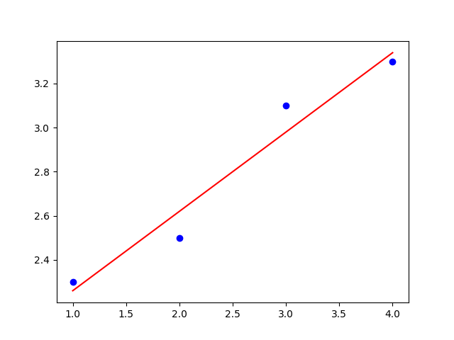
Exercise 5. Find the regression line for the given data.
| \(x\) | \(1{.}0\) | \(2{.}0\) | \(3{.}0\) | \(4{.}0\) |
|---|---|---|---|---|
| \(y\) | \(2{.}3\) | \(2{.}5\) | \(3{.}1\) | \(3{.}3\) |
Solution.
Let vectors \(\vec X\) and \(\vec Y\) be given by the first and second rows of the table, respectively. Then: \[ \begin{aligned} \vec X\cdot\vec X&=1{.}0^2+2{.}0^2+3{.}0^2+4{.}0^2=30,\cr \vec X\cdot\vec Y&=1{.}0\cdot 2{.}3+2{.}0\cdot 2{.}5+3{.}0\cdot 3{.}1+4{.}0\cdot 3{.}3=29{.}8,\cr \vec 1\cdot\vec X&=1{.}0+2{.}0+3{.}0+4{.}0=10,\cr \vec 1\cdot\vec Y&=2{.}3+2{.}5+3{.}1+3{.}3=11{.}2,\cr \vec 1\cdot\vec 1&=1+1+1+1=4. \end{aligned} \]
Substituting these values into system (3) gives: \[ \begin{aligned} 30a+10b&=29{.}8,\cr 10a+4b&=11{.}2. \end{aligned} \] Solving this system yields: \(a=0{.}36\) and \(b=1{.}90\). The regression line for the given data is therefore \[y=0{.}36x+1{.}90.\] The figure shows the regression line along with the data points.
Final Notes
- In statistics, the method described above is one of the fundamental tools used to predict whether one variable influences the values of another. For this reason, there are methods that evaluate the quality of the approximation and assess whether the chosen model is suitable for a given set of data points.
- There are also multivariable (multivariate) versions of the least squares method, where the predicted value depends not on a single, but on several independent variables.
- The problem of solving an inconsistent system of linear equations also appears in image reconstruction in acoustic tomography. This allows studying the composition of geological layers or the health of wood or a tree based on information about the speed at which elastic deformation waves pass through the material. A series of articles on the blog https://tomroelandts.com/ can serve as an introduction to the issue.
- It is also possible to derive direct formulas for calculating the coefficients of linear regression from the given data — this approach avoids computing dot products and solving systems of equations. See for example https://en.wikipedia.org/wiki/Simple_linear_regression#Expanded_formulas.
Literature and References
Literature
- Wikipedie, Simple linear regression, https://en.wikipedia.org/wiki/Simple_linear_regression, 12.4.2024
- Tom Roelandts, https://tomroelandts.com/articles/tomography-part-1-projections, https://tomroelandts.com/articles/the-sirt-algorithm, 13.4.2024
Sources of figures
- https://commons.wikimedia.org/wiki/File:Flag-map_of_the_United_States.svg
We will use a notation commonly used in data processing, where data sets (vectors) are denoted by capital letters and a vector that has all components equal to the same number is written as a given number with an arrow to indicate the vector.↩︎
Strictly speaking, this operation does not make mathematical sense, because we are adding a vector to a real number. This operation must be interpreted component-wise, where this addition means that the real number is changed to a vector of the appropriate dimension so that the operation is defined. We call this adaptation broadcasting. As a result, we add the value \(b\) to each component of the vector \(a\vec X\).↩︎
Be careful, the exercise is quite sensitive to rounding.↩︎
