
Rozmanitosť ekosystémov na ostrovoch
 30 min.,
  2/3
2/3 V tomto texte predvedieme dôležitosť logaritmov v biologických vedách. Život v prírode je neustálym bojom o prežitie. Zvieratá alebo rastliny musia zabezpečiť prežitie svojho druhu. U zvierat to zahŕňa schopnosti a sily na únik pred predátormi, prístup k potrave a dostupnosť miest na hniezdenie, rozmnožovanie a ochranu potomstva, kým nie je schopné žiť samostatne. Na dosiahnutie tohto cieľa je potrebný dostatočný životný priestor. Tieto požiadavky môžu byť splnené v oblasti s dostatočnými zdrojmi (potrava, miesta na hniezdenie atď.). Množstvo zdrojov úzko súvisí s veľkosťou oblasti. Biológovia poznaju zákon, ktorý definuje vzťah medzi počtom druhov trvalo žijúcich v ekosystéme a rozlohou tohto ekosystému. Tento zákon (angl. species-area relationship) má tvar \[N=c A^k,\tag{1}\] kde \(N\) je počet druhov, \(A\) je rozloha územia a \(c\) a \(k\) sú konštanty. Konštanta \(c\) závisí od jednotiek plochy a udáva teoretický počet druhov v oblasti s jednotkovou rozlohou. Konštanta \(k\) sa typicky pohybuje medzi \(0{,}2\) a \(0{,}35\) pre ostrovy a \(0{,}12\) až \(0{,}17\) pre pevninu. Vzťah (1) bol experimentálne potvrdený napríklad na mangrových ostrovoch pri Floride. Tieto malé ostrovy sú v podstate stromy rastúce zo slanej vody plytkeho mora. Vzhľadom na malé rozmery ostrova bolo možné študovať odozvu ekosystému na zmeny rozlohy ostrova. Výskumníci použili reťazovú pílu na zmenšenie rozlohy a pozorovali zodpovedajúci pokles počtu druhov. Dodatočne boli vykonané experimenty s kolonizáciou neobývaného ostrova. V takýchto prípadoch bol život na ostrove chemicky vyhubený podobne ako sa dezinfikujú domy. Výskumníci potom pozorovali, že bohatosť druhov sa spontánne vrátila do pôvodného stavu. Zaujímavé je, že počet druhov zostal rovnaký, ale konkrétne druhy boli nahradené inými. Keďže vzťah (1) je mocninová funkcia s všeobecným neceločíselným exponentom, nie je závislosť medzi rozlohou ekosystému a počtom druhov jednoducho identifikovateľná z nameraných alebo pozorovaných údajov. Napriek tomu je poznanie tohto funkčného vzťahu dôležité. Pomáha nám to napríklad v ochrane prírody. Ekosystém v uvedenom kontexte je väčšinou ostrov, ale v skutočnosti znamená zovšeobecnený ostrov. Pod ostrovom nerozumieme len pevninu obklopenú morom, ale akúkoľvek oblasť umiestnenú do územia iného typu. Napríklad ostrovom môže byť jazero v rámci pevniny, malý les v poľnohospodárskej krajine alebo chránená krajinná oblasť obklopená územím s bežným režimom. Poznanie toho, ako veľkosť oblasti súvisí so zložením a diverzitou druhov, je dôležitým faktorom pri rozhodovaní, či vybudovať jednu veľkú prírodnú rezerváciu alebo niekoľko malých na ochranu prírody. S podobným zákonom ako je vzťah (1) sa v biológii stretávame veľmi často v alometrických vzťahoch. Toto sú vzťahy, kde sa fyzikálne a fyziologické vlastnosti organizmov menia v závislosti od veľkosti organizmu. Napríklad vzťah medzi časom potrebným na dosiahnutie dospelosti a telesnou hmotnosťou má podobnú formu, viď Begon (1997). Ďalším príkladom je Kleiberov zákon, ktorý spája hmotnosť zvieraťa a jeho bazálny metabolizmus. V nasledujúcich úlohách vyriešime zadania súvisiace so vzťahom (1) a ukážeme, ako používať logaritmy pri práci s ním.
Úlohy
Úloha 1: Ukažte, že po zlogaritmovaní vzťahu (1) je výsledná závislosť lineárna, t. j. pokiaľ na osi nanesieme namiesto veľkosti územia a počtu druhov ich logaritmy, tak grafom závislosti bude priamka.
Riešenie. Vychádzame zo vzťahu (1), t. j. \[N=c A^k.\]
Logaritmovaním dostaneme
\[\log N= \log (c A^k).\]
Použitím pravidla pre logaritmus súčinu a logaritmus mocniny dostaneme
\[\log N= \log (c) + k\log A.\]
Substitúcie \(y=\log N\), \(q = \log c\), \(x=\log A\) transformujú rovnicu na
\[y=kx+q,\]
čo je rovnica priamky so smernicou \(k\).
Poznámka: Keďže nie je vždy pohodlné počítať dva logaritmy pre každú hodnotu pri kreslení grafu, používajú sa takzvané logaritmické osi. Na logaritmickej osi je vzdialenosť medzi bodom \(x\) a bodom 1 určená hodnotou \(\log x\), pričom rovnaká logaritmická mierka platí pre horizontálnu aj vertikálnu os.
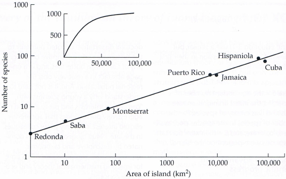
Priložený obrázok ukazuje, ako sa pri použití logaritmických osí mení mocninová závislosť na lineárnu. Graf zahŕňa počet druhov plazov a obojživelníkov na ostrovoch v Západnej Indii (angl. West Indies, Antily a Bahamy). V grafe s logaritmickými osami sa údaje zarovnávajú takmer presne do priamky. Táto vlastnosť je ľahko viditeľná v údajoch a môže byť tiež ľahko potvrdená matematickými metódami. Vložený menší obrázok ukazuje, ako by závislosť vyzerala bez použitia logaritmických osí. Údaje ležia pozdĺž krivky a nie je okamžite jasné, či je to mocninová krivka, exponenciálna krivka alebo nejaká iná závislosť.
Úloha 2: Odhaduje sa, že pre určitú oblasť je hodnota exponentu \(k\) rovná \(0{,}15\). O koľko sa zníži počet druhov, ak sa rozloha zmenší na jednu desatinu? Táto úloha modeluje napríklad rozsiahle vyťažovanie lesa.
Riešenie. Vychádzať budeme zo vzťahu \[N(A)=c A^k\] a zmenšíme rozlohu na jednu desiatu, potom dostaneme \[N(0{,}1A) = c\cdot(0{,}1 A)^k = c A^k \cdot 0{,}1^k = N(A)\cdot 0{,}1^k\] Odtiaľ pre \(k=0{,}15\) dostaneme \[\frac{N(0{,}1A)}{N(A)}=0{,}1^k = 0{,}71.\] Po zmenšení rozlohy na jednu desatinu sa počet druhov zvierat zníži na 71 percent pôvodného stavu, t. j. zníži sa o 29 percent.
Úloha 3: Bolo pozorované, že po zmenšení rozlohy na jednu štvrtinu sa počet druhov znížil na sedemdesiat percent pôvodného stavu. Odhadnite hodnotu parametra \(k\).
Riešenie. Označíme pôvodné hodnoty pre rozlohu a počet druhov ako \(A_1\) a \(N_1\). Nové hodnoty budú \(A_2\) a \(N_2\). Oba súbory údajov spĺňajú rovnicu (1), preto \[N_1 = c A_1^k\] a \[N_2 = c A_2^k.\] Delením týchto rovníc dostaneme \[\frac{N_1}{N_2} = \frac{c A_1^k}{ c A_2 ^k} =\left(\frac {A_1}{A_2}\right)^k.\] Podľa zadania platí \(N_2=0{,}7N_1\) a \(A_2=0{,}25A_1\) t. j. \[\frac{N_1}{0{,}7N_1}=\left(\frac{A_1}{0{,}25A_1}\right)^k\] \[\frac{1}{0{,}7}=\left(\frac{1}{0{,}25}\right)^k.\] Logaritmovaním oboch strán dostaneme \[\log\frac{1}{0{,}7}=k\cdot\log\frac{1}{0{,}25}.\] a teda \[k=\frac{\log \frac1{0{,}7}}{\log 4}\approx 0{,}257.\]
Literatúra
- Teorie ostrovní biogeografie, ENVI WIKI, https://www.enviwiki.cz/w/index.php?title=Teorie_ostrovn%C3%AD_biogeografie, October 3, 2023
- Co je ostrovní biogeografie?, https://zemepisec.cz/biogeografie/ostrovni/, October 3, 2023
- Species–area relationship, Wikipedie, https://en.wikipedia.org/wiki/Species%E2%80%93area_relationship, October 3, 2023
- Culek M., Biogeografie, https://is.muni.cz/el/1431/jaro2010/Z0005/18118868/index_book_3-1-1.html, October 3, 2023
- Begon, M. et al. Ekologie: jedinci, populace a společenstva : [Investice do rozvoje vzdělávání, reg.č.: CZ1.07/2.2.00/15.0084]. 1st ed. Olomouc: Vydavatelství Univerzity Palackého, 1997. 949 p. ISBN 80-7067-695-7.
