When an Acoustic Tomograph Meets a Resistograph

15 min., 1/3

You might not expect it, but analytic geometry plays a role in monitoring the health of trees. Trees are an essential part of the urban environment. However, assessing their condition can be challenging—especially when there are no visible signs of damage. Analytic geometry provides an effective way to link different diagnostic methods and create a unified model that helps evaluate the risk of a tree falling. This enables more informed decisions regarding tree care and potential intervention.

The Issue of Trees in Urban Areas

Trees are an important element that makes life in urban environments more pleasant. They provide shade and oxygen, reduce dust and noise, lower the surrounding temperature, and offer shelter for birds and other animals.

However, planting trees in urban areas also comes with certain risks. One of the most serious is the risk of a tree falling. A falling tree can injure people, damage property, or—at worst—cause death. That is why it is essential to regularly monitor the health of trees and detect potential issues in time.

Tree Diagnostics

Arborists—specialists in the care of trees outside of forests—use various methods to assess tree health. One of these methods is the acoustic tomograph, which allows for a non-invasive evaluation of the wood inside the trunk without damaging the tree. It works much like a CT scan for trees, revealing hidden defects and wood decay. Unlike medical CT scans, however, an acoustic tomograph uses sound waves with long wavelengths, which comes with limitations based on the physical principles of wave propagation. One consequence is that the acoustic tomograph cannot reliably distinguish between a hollow and a crack inside the tree. Both defects appear as areas where sound travels more slowly than in the surrounding healthy wood. Cracks are often overestimated in size and may look similar to cavities in the resulting image. For this reason, it is recommended to use additional diagnostic tools to gain a more complete understanding of the tree’s condition.

One such tool is the resistograph, which measures the stiffness of wood and helps detect hidden defects. The resistograph uses a fine drill and measures the resistance of the wood to assess its structure and mechanical properties. Because the drill is extremely thin, this method is only minimally invasive and causes little to no harm to the tree. The resistograph can detect cracks, cavities, and other internal defects. The data it provides can complement the findings from the acoustic tomograph.

In practice, tree diagnostics usually begin with measurements taken using an acoustic tomograph, which provides basic information about the condition of the wood inside the trunk. This is typically followed by measurements with a resistograph, which offers additional insight and helps detect hidden defects. By combining both methods, it is possible to create a comprehensive picture of the tree’s health and detect potential issues early.

The figure below shows example outputs from an acoustic tomograph and a resistograph. On the left is a reconstruction from the acoustic tomograph, displaying the speed of sound propagation through the wood. This speed is important because it directly relates to the mechanical properties of the wood. Blue and red areas represent zones where the sound travels more slowly; in the green areas, the sound moves faster. On the right is the output from the resistograph, which shows the power required to maintain a constant drill speed—this serves as an indicator of the wood’s mechanical strength. Each drill measurement was taken between two sensors of the acoustic tomograph, meaning that twelve drillings were performed between the twelve tomograph sensors.

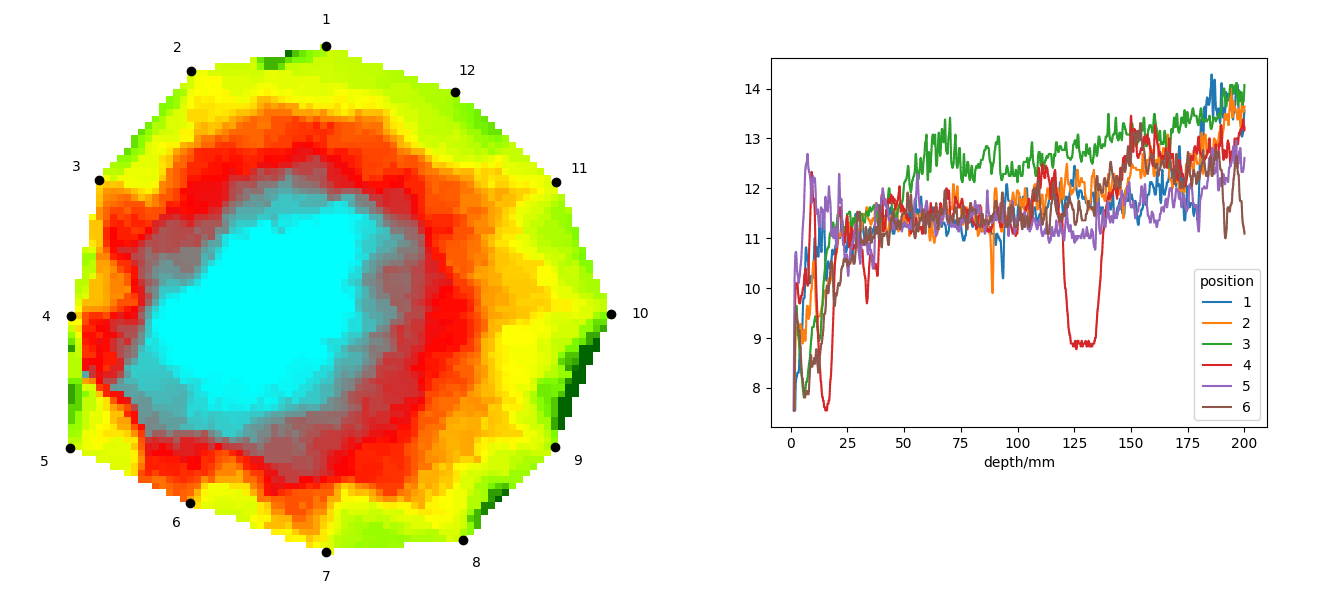
The image shows that one of the resistograph curves has a noticeable drop at a depth of approximately 125 millimeters. This drop corresponds to a cavity about one centimeter in size. However, the acoustic tomograph indicates a larger cavity. To make data processing easier, it is helpful to combine the data into a single image. For this reason, we would like to include both the drill locations and resistograph readings in the tomogram (the output from the acoustic tomograph).

Combining Data from the Acoustic Tomograph and the Resistograph

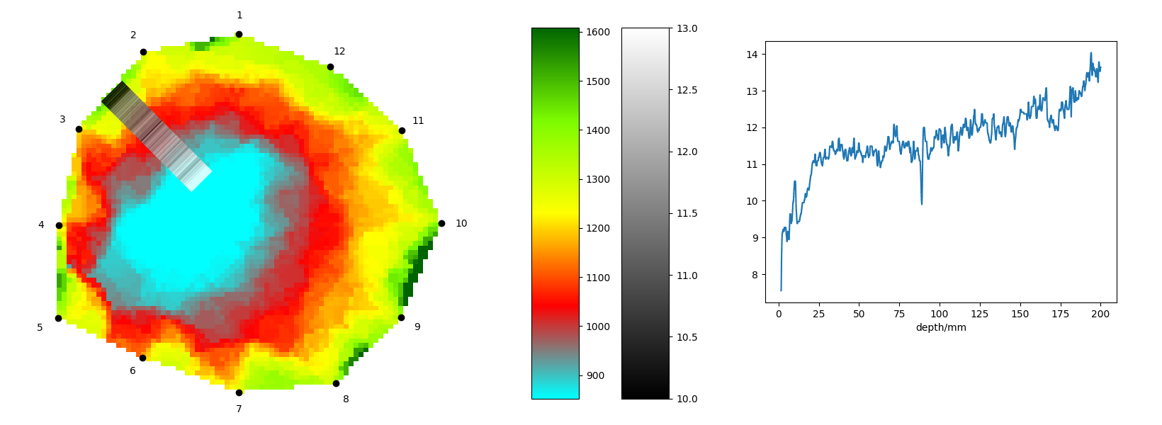
The process of combining data from both methods requires the use of mathematics. Let’s assume that the drilling was done from the midpoint between two adjacent sensors and directed toward the center of the tree trunk. We will represent the resistograph readings using grayscale intensity, and the final image will be a composition of the tomogram and a column with varying grayscale intensity.

The tomogram is typically placed in a coordinate system so that its center lies at the origin, the first sensor is located on the positive part of the \(y\)-axis, and the remaining sensors are numbered counterclockwise. To create a column of resistograph data between the second and third sensors, we need a mathematical function that maps the depth value from the resistograph curve to a position in the tomogram’s coordinate system. The graph of this function will be a straight line extending from the midpoint between the two sensors to the center of the tree. Let’s denote this line as \(p\).

The steps to find a suitable equation for line \(p\) may be as follows:

• First, determine the coordinates of the midpoint between the two sensors. Let this point be \(A\). The line \(p\) must pass through point \(A\).
• Next, determine the direction vector \(\vec u\) of line \(p\). This will be the vector pointing from point \(A\) to the origin of the coordinate system.
• Using point \(A\) and the direction vector \(\vec u\), we can write the parametric equation of line \(p\). However, this approach would require establishing a connection between the parameter in the equation and the drilling depth. If we instead convert the direction vector \(\vec u\) into a unit vector, denoted \(\vec e\), the parameter in the line equation will directly correspond to the drilling depth. Therefore, we first find the vector \(\vec e\) as the unit vector in the direction of vector \(\vec u\).
• The parametric equation of the line defined by point \(A\) and vector \(\vec e\) gives a mapping from drilling depth to coordinates in the tomogram’s coordinate system. This function can then be used to overlay resistograph data onto the tomogram.

Let’s try this procedure on a specific example based on the geometry shown in Figure 1.

Solution. The midpoint \(A\) of the line segment between points \(P_2\) and \(P_3\) is calculated using the formula

\[ A = \frac{P_2 + P_3}{2}.\]

Substituting the coordinates, we get \(A=[-20, 20]\).

The direction vector \(\vec u\) of the line \(p\) is determined using the points \(O\) and \(A\) that lie on the line: \[\vec u = O-A,\] which in coordinates gives \(\vec u = [0,0] - [-20, 20] = (20, -20)\).

The magnitude of the vector \(\vec u=(u_1, u_2)\) is calculated using the Pythagorean theorem: \[|\vec u| = \sqrt{u_1^2 + u_2^2} = \sqrt{20^2 + (-20)^2} = \sqrt{800} = 20\sqrt{2}.\]

The unit vector \(\vec e\) in the direction of vector \(\vec u\) is given by dividing the vector by its magnitude: \[\vec e = \frac{\vec u}{|\vec u|} = \left(\frac{20}{20\sqrt{2}}, \frac{-20}{20\sqrt{2}}\right) = \left(\frac{1}{\sqrt{2}}, \frac{-1}{\sqrt{2}}\right).\]

The final parametric equations of line \(p\) are therefore: \[ \begin{align*} x &= -20 + t \cdot \frac{1}{\sqrt{2}}, \\ y &= 20 - t \cdot \frac{1}{\sqrt{2}}, \qquad t\in\mathbb R. \end{align*} \]

Solution. We need to replace the vector \(\vec u\) with a direction vector that is perpendicular to the segment defined by the acoustic tomograph sensors. Vectors that are perpendicular to a given vector \(v = (v_1,v_2)\) are \((-v_2,v_1)\) and \((v_2,-v_1)\). The vector from point \(P_2\) to point \(P_3\) has coordinates \[ \vec v = P_3 - P_2 = (-25, 14) - (-15, 26) = (-10, -12). \] In our case, the two perpendicular direction vectors are \[ \vec n_{1} = (12, -10), \quad \vec n_{2} = (-12, 10). \] From Figure 2, it is clear that the direction vector should point to the right and downward, so we use the vector \(\vec n_{1}\). The magnitude of vector \(\vec n_{1}\) is \[ |\vec n_{1}| = \sqrt{12^2 + (-10)^2} = \sqrt{244} = 2\sqrt{61} \] and the unit vector in the direction of \(\vec n_{1}\) is obtained by dividing the vector by its magnitude: \[\vec e = \frac{\vec n_{1}}{|\vec n_{1}|} = \left(\frac{12}{2\sqrt{61}}, \frac{-10}{2\sqrt{61}}\right) = \left(\frac{6}{\sqrt{61}}, \frac{-5}{\sqrt{61}}\right).\]

The parametric equations of the line \(p\) are therefore: \[ \begin{align*} x &= -20 + t \cdot \frac{6}{\sqrt{61}}, \\ y &= 20 - t \cdot \frac{5}{\sqrt{61}}, \qquad t\in\mathbb R. \end{align*} \]

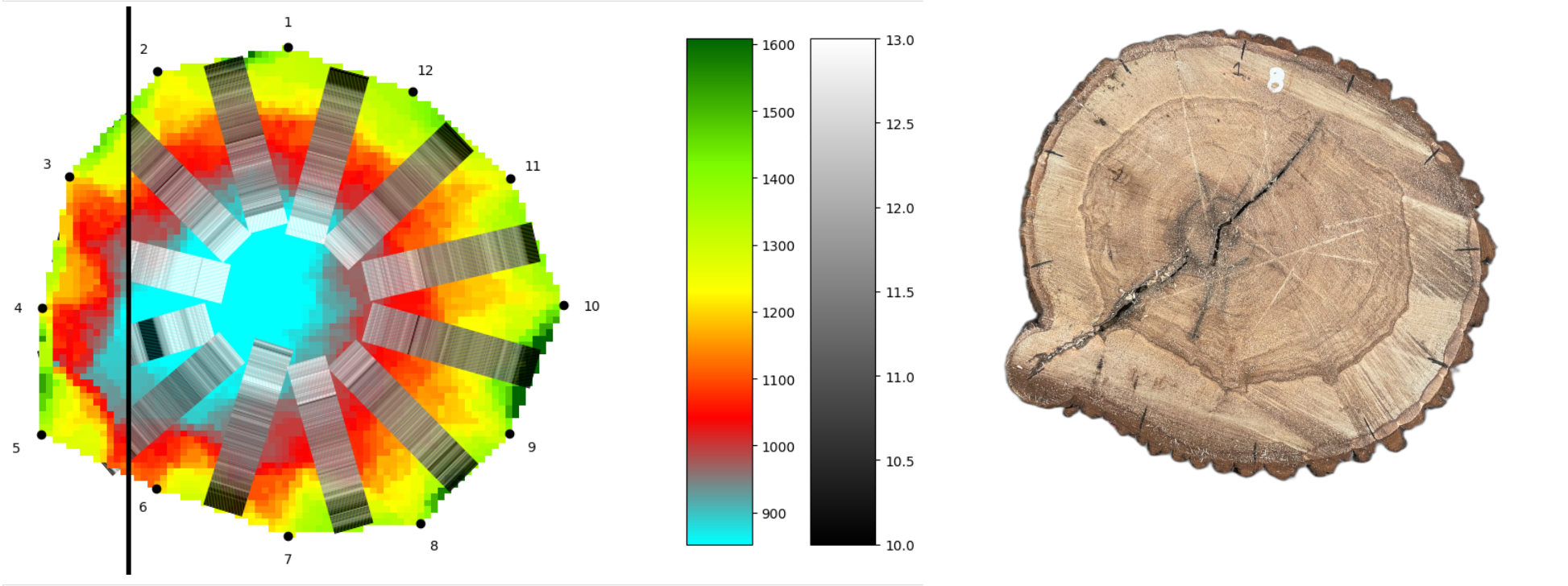
Note. The procedure described in the previous problems can be applied to any pair of acoustic tomograph sensors and can be easily implemented in an algorithm. The result is a combined visualization of resistograph and acoustic tomograph data in a single image.

Data Source

The data and photos in this text come from real measurements carried out on trees in the Valdštejn Linden Alley in Jičín. This is the oldest linden tree avenue in the Czech Republic, with a length of over 1,700 meters. Since not all of the trees are in good health, regular monitoring is necessary. As part of the monitoring process, some trees were selected for felling, and measurements were performed on them beforehand. This provided a unique opportunity to compare the diagnostic results with the actual condition of the trees. The measurements were conducted by arborist Vojtěch Semík, and the data were processed as part of the ERC CZ project DYNATREE (https://starfos.tacr.cz/cs/projekty/LL1909).

Conclusion

In this text, we explored how tools from analytic geometry can be applied to combine data from an acoustic tomograph and a resistograph. We demonstrated how to use a parametric equation of a line to convert drilling depth data from the resistograph into coordinates in the tomograph’s coordinate system. This method can improve the accuracy of tree health assessments and provide a more complete picture of the internal condition of the wood. By merging data from both diagnostic tools, it is possible to detect hidden defects more reliably—an essential step for maintaining tree health and ensuring safety in urban environments.

Literature and References

Literature

1. https://rinntech.info/products/resistograph/ (online, accessed June 6, 2025)
2. https://www.kudyznudy.cz/aktivity/valdstejnska-lipova-alej-v-jicine-nejstarsi-doch (online, accessed June 6, 2025)
3. https://www.jicin.org/lipova-alej (online, accessed June 6, 2025)
4. https://zpravyceskyraj.cz/stromy-vedi-co-a-proc-delaji-arborista-vojtech-semik-o-jicinske-lipove-aleji/ (online, accessed June 6, 2025)

Image Sources

1. Project DYNATREE – Tree Dynamics: Understanding of Mechanical Response to Loading, https://starfos.tacr.cz/cs/projekty/LL1909.
2. Author’s own images