
Tree Tomography
 30 min.,
  2/3
2/3 Knowing the health condition of a tree is important, for example in city parks, where public safety is a concern. Inspections focus mainly on older trees, as these are more likely to be unhealthy. The trunk of a damaged or diseased tree can break in strong winds, causing injury or property damage. Similarly, owners of smaller properties may have an old tree near their house and do not want to risk it falling and damaging, for instance, the roof.
A tree’s health can be assessed by an arborist, who checks whether the tree is thriving or beginning to dry out. The arborist looks for wood-decaying fungi around the trunk, as well as for areas that are visibly damaged. Their observations can be supported by using a tree tomograph or a pull test. Based on the findings, the arborist may suggest various safety measures—such as pruning branches in the crown to reduce strain on the trunk during strong winds.
Common non-invasive methods for assessing a tree’s health include the pull test and acoustic tomography using a tree tomograph.
Pull Test
This test is based on measuring how a tree reacts when its trunk is slightly tilted. In practice, a rope is tied to the trunk at a certain height and pulled. Sensors placed at the base of the trunk record the resulting response. The arborist compares the results with known response patterns for different tree species to evaluate the specific case. The goal is to determine the condition of the tree’s root system and whether the trunk is at risk of breaking. This method is relatively expensive. The measurement takes quite a long time and also requires a tree climber to tie the rope to the tree and remove it afterward. For these reasons, the method is now used less often and has been largely replaced by tree tomography.
Tree Tomography
The tree tomograph works on the principle of sound transmission. Sensors with small spikes are placed around the trunk at a certain height. The spikes are gently hammered through the bark into the wood. They are always inserted into the tree’s active tissue, where regeneration is fast. This way, the tree is not harmed by the procedure.
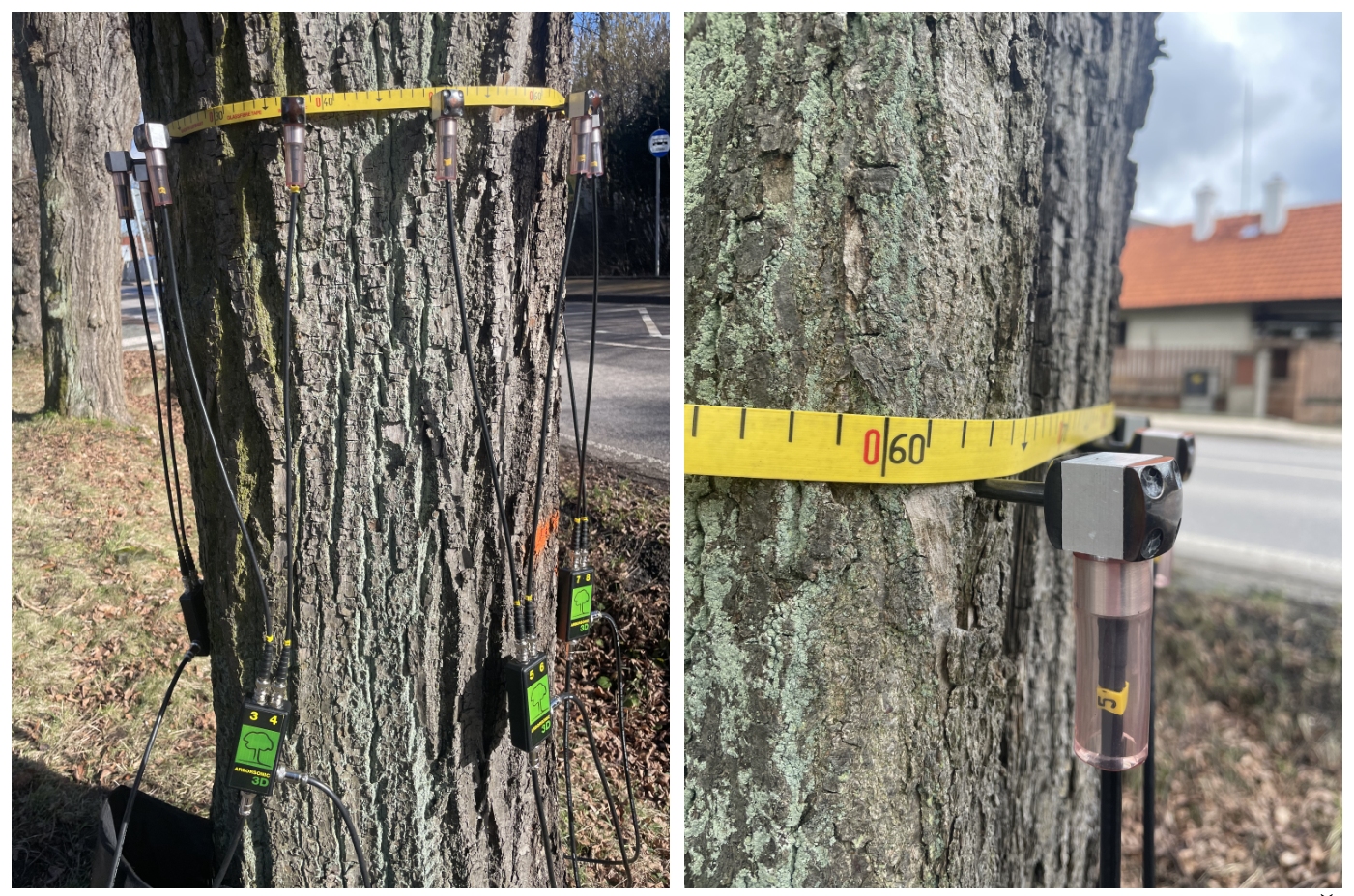
The arborist then gently taps on each sensor with a small hammer. While doing this, the system measures how quickly the sound signal travels to the other sensors. Sound moves quickly through healthy wood, but slows down when it passes through internal defects. By comparing the measured values to reference data, it is possible to detect issues such as cavities inside the tree at an early stage.
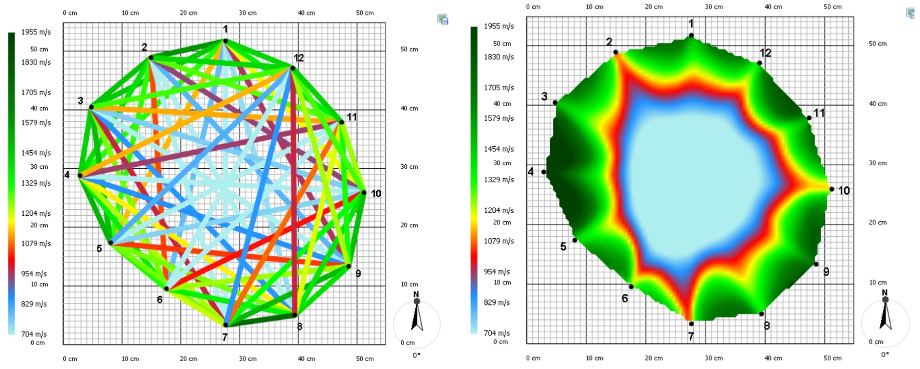
The measured sound transmission speeds can be used to create a so-called velocity graph (see Figure 3). The color of the line segments connecting the individual points is important—it indicates the speed at which the sound signal travelled from one point to another. A computer program then uses these measured speeds to generate a result called a tomogram. This is a two-dimensional image that shows zones with different sound transmission properties.
To assess the condition of a tree, the arborist does not measure just one cross-section, but several—focusing on visibly damaged areas of the trunk. Based on all the collected information, the arborist forms an overview of the tree’s overall health.
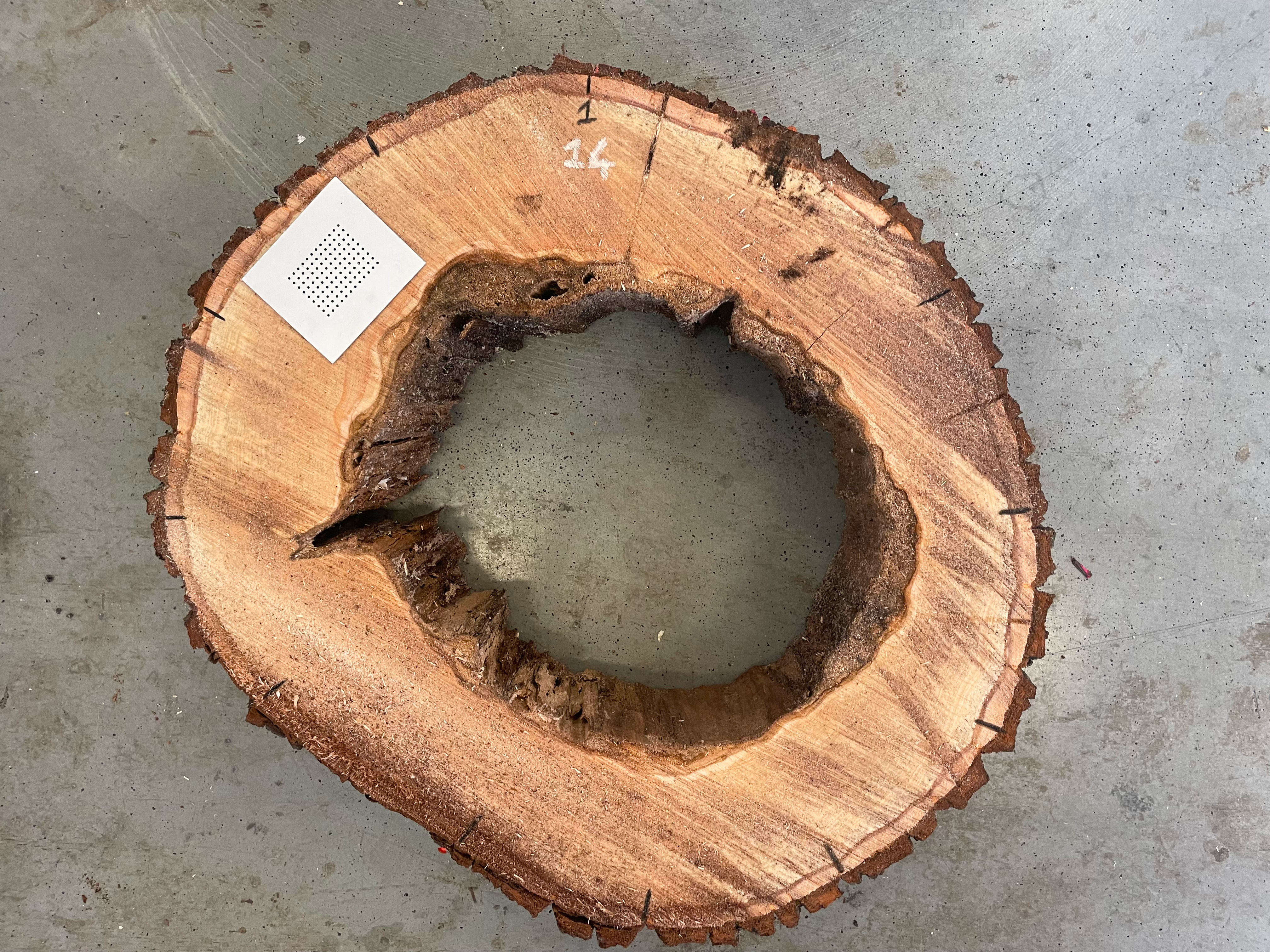
The presence of a cavity in the trunk does not necessarily indicate a serious problem, as long as the outer part of the trunk remains healthy. It is not possible to define exactly how much healthy wood must surround the cavity—this depends on the type of wood, the age of the tree, and the diameter of the trunk. The principle is similar to that of a steel pipe, which remains strong even if it is hollow, as long as the material is intact around the outer edge. There are several guidelines. One states that it is acceptable if one third of the trunk’s cross-section is healthy. Another suggests that for very old trees, even a 3-centimeter ring of healthy wood around the perimeter may be sufficient.
A tree tomograph can be used to fairly accurately assess the condition of the root system. Measurements are taken right at ground level and then at several higher points along the trunk. If the results show that rot is spreading upward from the base of the trunk, it is likely that the roots are also compromised.
Even a tomograph has its limitations. Measurements are not taken during winter when temperatures are below freezing, because frozen sap changes how sound travels through the wood, which could distort the results.
To construct a tomogram, the distances between all the sensors used must be known. These distances can usually be measured using calipers. However, with very old and massive trees, using calipers can be problematic—the tool may simply not be long enough. So what can be done when it’s not possible to measure all the required distances between sensors? For simplicity, we will now limit the problem to distances between just four sensors.
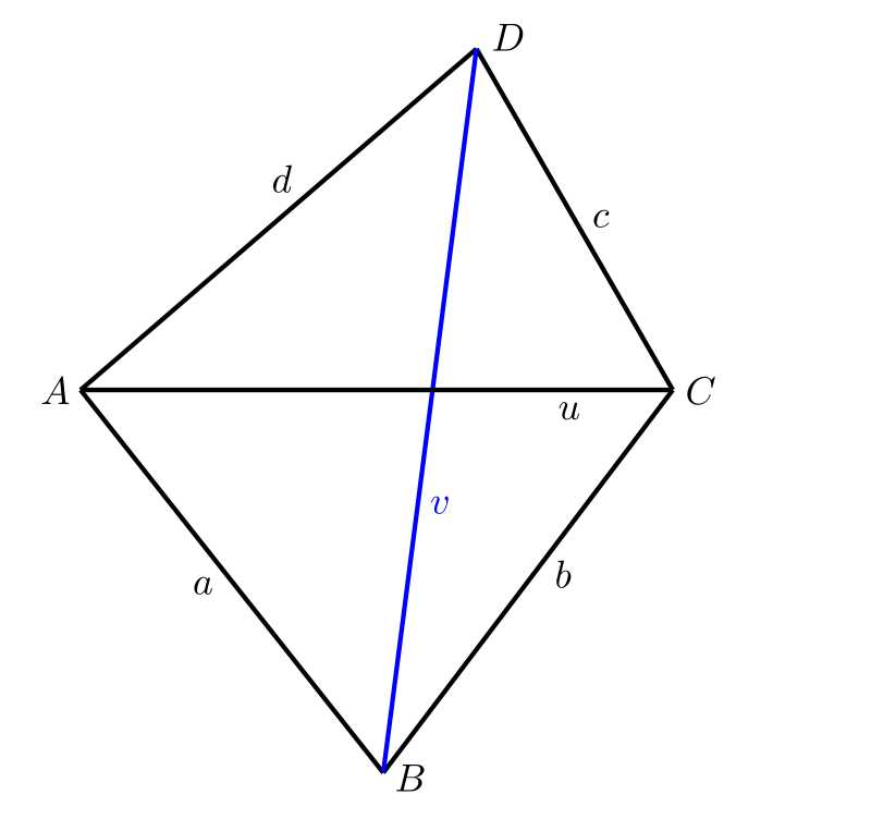
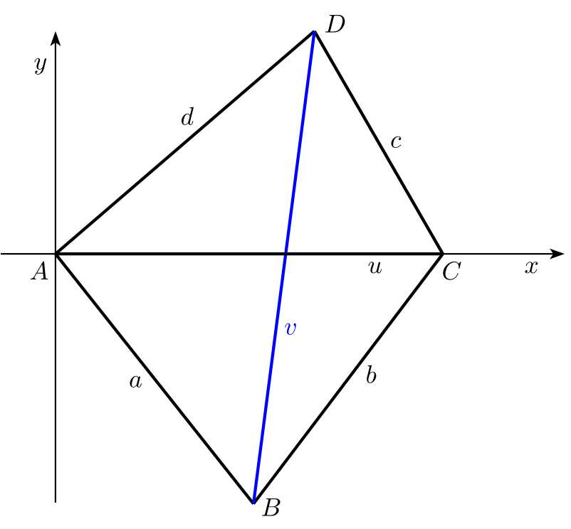
Exercise 1. Let us consider a general quadrilateral \(ABCD\). In this quadrilateral, we know the lengths of all four sides \(a\), \(b\), \(c\), and \(d\), as well as the length \(u\) of one diagonal \(AC\). The length \(v\) of the other diagonal \(BD\) is too large to be measured with our measuring device. How could we construct this length?
Solution. The geometric solution is of course the simplest. We first draw the segment \(AC\). Since we know the lengths of sides \(AB\) and \(BC\), we can construct triangle \(ABC\) on the diagonal \(AC\). In the same way, we construct triangle \(ADC\), and then we only need to measure the length of the diagonal \(BD\). In practice, this is done using an appropriate scale.
A solution drawn by hand on paper will not be very accurate. However, if we construct the same figure using a geometric drawing program on a computer (for example, GeoGebra), the precision of the result will be sufficient.
The problem arises when the arborist needs to perform this calculation not just once, but many times. In that case, a geometric solution would become time-consuming and inefficient. It would be better to have a program—an Excel spreadsheet would be enough—where the measured values could be entered, and the missing length would be calculated by the computer.
Exercise 2. Solve the problem from Exercise 1 analytically.
Solution. We begin by choosing a suitable coordinate system. We place the origin at point \(A\) and choose the \(x\)-axis so that point \(C\) lies on it. With this setup, the coordinates of the quadrilateral’s vertices are: \[A[0, 0],\; C[u, 0],\; B[b_1, b_2],\; D[d_1, d_2].\]
We need to determine the coordinates \(b_1\), \(b_2\), \(d_1\), and \(d_2\). After that, it will be easy to calculate the desired length of diagonal \(v\) as the magnitude of the vector \(\overrightarrow{BD}\).
We will first work with triangle \(\bigtriangleup ACD\) to determine the coordinates of point \(D\). We will find the vectors \(\overrightarrow{AD}\) and \(\overrightarrow{CD}\).
\[ \begin{aligned} & \overrightarrow{AD} = D-A = (d_1,d_2),\\ & \overrightarrow{CD} = D-C = (d_1-u,d_2) \end{aligned} \] and calculate their magnitudes \[ \begin{aligned} & \|\overrightarrow{AD}\| = \sqrt{d_1^2+d_2^2} = d,\\ & \|\overrightarrow{CD}\| = \sqrt{(d_1-u)^2+d_2^2} = c. \end{aligned} \] By squaring the expressions, we obtain a system of two equations with two unknowns, \(d_1\) and \(d_2\) \[ \begin{aligned} & d_1^2+d_2^2 = d^2,\\ & (d_1-u)^2+d_2^2 = c^2. \end{aligned} \] We can solve the system using, for example, the addition method. By multiplying the second equation by \(-1\) and adding both equations, we get: \[2d_1u-u^2=d^2-c^2.\] From this equation, we express: \[d_1=\frac{1}{2u}(d^2-c^2+u^2).\] Substituting \(d_1\) into the first equation gives: \[d_2^2=d^2-d_1^2,\] and by taking the square root, we find: \[d_2=\sqrt{d^2-d_1^2}.\]
In a similar way, we use triangle \(\bigtriangleup ABC\) to calculate the coordinates of point \(B\). We work with the vectors \(\overrightarrow{AB}\) a \(\overrightarrow{CB}\). The vectors \[ \begin{aligned} & \overrightarrow{AB} = B-A = (b_1,b_2),\\ & \overrightarrow{CB} = B-C = (b_1-u,b_2) \end{aligned} \] have the magnitudes \[ \begin{aligned} & \|\overrightarrow{AB}\| = \sqrt{b_1^2+b_2^2} = a,\\ & \|\overrightarrow{CB}\| = \sqrt{(b_1-u)^2+b_2^2} = b. \end{aligned} \] By squaring the expressions, we obtain a system of two equations for the two unknowns \(b_1\) and \(b_2\). \[ \begin{aligned} & b_1^2+b_2^2 = a^2,\\ & (b_1-u)^2+b_2^2 = b^2. \end{aligned} \] From this we get: \[b_1=\frac{1}{2u}(a^2-b^2+u^2).\] From the first equation, we get: \[b_2^2=a^2-b_1^2\] and by taking the square root: \[b_2=-\sqrt{a^2-b_1^2}.\] The negative sign in the last equation is due to the fact that point \(B\) has a negative \(y\)-coordinate (points \(B\) and \(D\) lie in opposite half-planes defined by the line \(AC\)).
We can now calculate the desired length of diagonal \(v\) as the magnitude of the vector \(\overrightarrow{BD}\) using the formula \[ v=\|\overrightarrow{BD}\| = D-B = \sqrt{(d_1-b_1)^2+(d_2-b_2)^2}. \]
Exercise 3. What complications arise when sensor \(Z\) is added to the setup? Again, we know the distances \(m\) and \(n\) from sensor \(Z\) to sensors \(A\) and \(D\), and we want to determine the distance from point \(Z\) to point \(B\)—that is, the length of another unmeasurable diagonal.
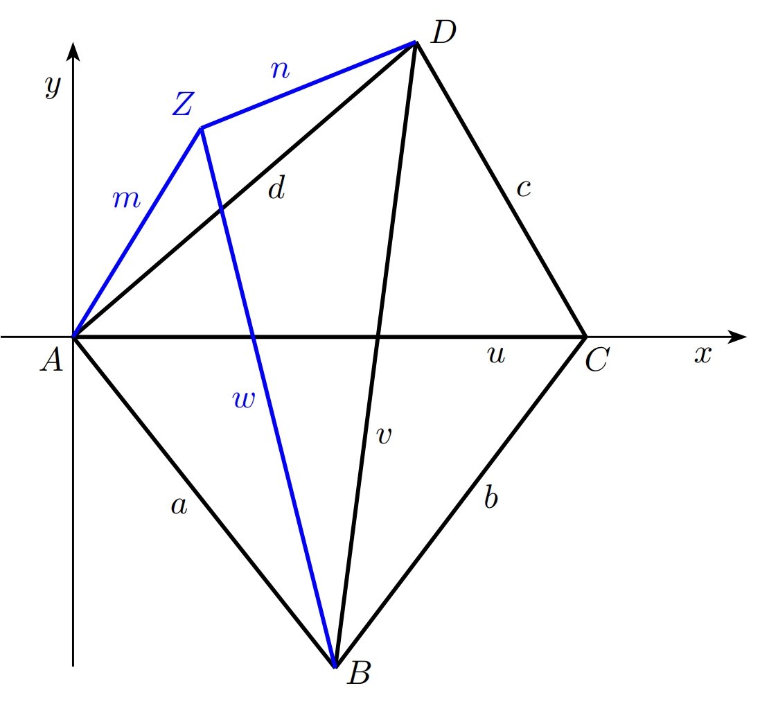
Solution. The procedure is the same as in Exercise 2, but this time we work with quadrilateral \(ABDZ\). In this quadrilateral, we know the lengths of all sides (let \(n\) be the length of side \(DZ\), and \(m\) the length of side \(ZA\)), as well as the length of diagonal \(AD\). Our goal is to determine the length of the other diagonal, denoted by \(w\).
Once again, it is helpful to choose a convenient coordinate system. We place the origin at point \(A\), and let the positive \(x\)-axis go through point \(D\). In this coordinate system, the vertices of the quadrilateral have the following coordinates: \[A[0,0],\;B[b_1,b_2,\;D[d,0],\;Z[z_1,z_2].\]
We get \[ \begin{aligned} & z_1 = \frac{1}{2d}(m^2-n^2+d^2),\\ & z_2 = \sqrt{m^2-z_1^2},\\ & b_1 = \frac{1}{2d}(a^2-v^2+d^2),\\ & b_2 = -\sqrt{a^2-b_1^2}. \end{aligned} \] From here, we can calculate the length of the diagonal \(w\) as the magnitude of the vector \(\overrightarrow{BZ}\) \[w=\|\overrightarrow{BZ}\|=\sqrt{(z_1-b_1)^2+(z_2-b_2)^2}.\]
Links and Literature
Literature
- iDNES.cz. Speciální tomograf odhalí nemocný strom. Nejtěžší je vyhodnotit výsledky [online]. Dostupné z https://www.idnes.cz/hobby/zahrada/stromovy-tomograf-mereni-zdravi-stromu.A190226_103850_hobby-zahrada_bma [cit. 21.,6.,2024].
- Thinktrees. Interpreting Arbotom sonic tomography results – Example no.1 [online]. Dostupné z https://thinktrees.co.uk/interpreting-arbotom-sonic-tomography-results-example-no-1/ [cit. 21.,6.,2024].
Source of Images
- Projekt DYNATREE – Tree Dynamics: Understanding of Mechanical Response to Loading, https://starfos.tacr.cz/cs/projekty/LL1909.
